Midpoint Report

Introduction

Food stands for any item that serves as a source of nutrition for a living organism. Being omnivores and apex predators, humans eat foods that come in all sorts of shapes, sizes, textures, and flavors [1]. Similarly, humans have vastly different preferences for which foods they’d rather consume. Still, there exists foods that are ubiquitously popular across the world. Ask any person if they are willing to pass up a sweet scoop of ice cream or perhaps a juicy, well-seasoned hot dog.

Generally, humans are quick to identify and fixate upon their favorite foods in their visual field. The Mattijs/snacks dataset is a collection of images of popular food items derived from the Google Open Images dataset, and is accompanied in textbooks such as Machine Learning by Tutorials [2, 4]. Give a human this dataset, and they can effortlessly classify which food is which. However, many people who are visually impaired may struggle with the crucial task of identifying what they are consuming. A program to identify everyday foods, such as apples or cookies, may prove to be useful for such individuals.

Problem Definition

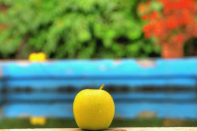
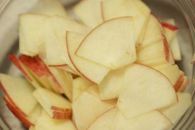
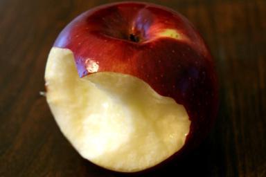
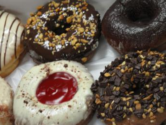
Identifying food items purely from visual appearance is surprisingly non-trivial. Here are examples of “apples” in the snacks dataset:

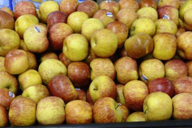Even with just one label, “apples” come in different forms, colors, and counts. Our objective is to make a machine learning model that can accurately classify the main type of food/snack apparent in an input image while generalizing to the variety of appearances that such an item can take. Since the project proposal, we have decided to move forward with the classification problem regarding the snacks dataset.

Methods

Data Collection

The snacks dataset has 20 different class labels of various different foods. The classes are as follows: ‘apple’, ‘banana’, ‘cake’, ‘candy’, ‘carrot’, ‘cookie’, ‘doughnut’, ‘grape’, ‘hot dog’, ‘ice cream’, ‘juice’, ‘muffin’, ‘orange’, ‘pineapple’, ‘popcorn’, ‘pretzel’, ‘salad’, ‘strawberry’, ‘waffle’, ‘watermelon’.

The photos in the dataset are of various dimensions. However, the images were scaled by the author of the dataset such that the smallest side is 256 pixels.

The dataset is pretty balanced as is. Most of the labels have about 350 images, with some exceptions in the popcorn and pretzel class. The dataset has already split the dataset into a train, validation, and test split, but we will merge the test and validation sets in case we plan to perform a custom cross validation technique in the future. Below is the number of data instances for each split that came with the dataset:

Set/Split	Count
Train	4838
Validation	955
Test	952
Total	6745

The train set after merging both splits from the Snacks dataset has a size of 5793 instances. Here is the breakdown of the training set:

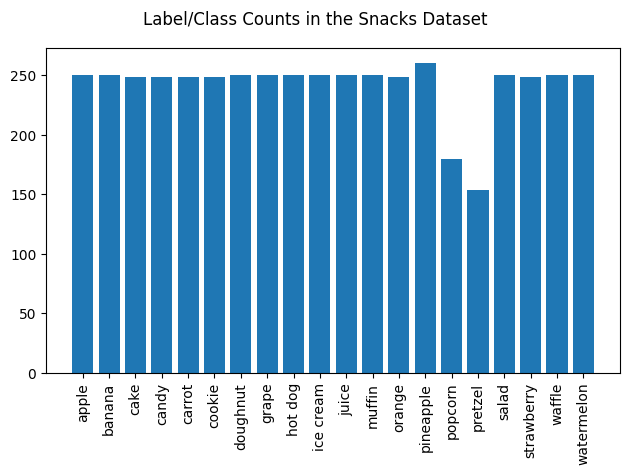
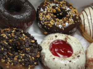
As we can see, now most of the classes have 300 examples. However, we’d ideally want the number of images in each class to basically be even. Additionally, it would be beneficial if we had more data to train on. We can generate more training data with data augmentation, a process in which more training data is generated from existing training data by slightly modifying existing images. Some of the transformations we decided to implement were scaling, rotating, cropping, and mirroring. For instance, take the following image, originally sampled from the training set:

We implement a scaling method, which simply makes the image smaller or larger on a uniform scale between 0.8 times and 1.2 times.

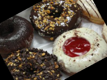
Our rotation method rotates the image anywhere from 0 to 180 degrees counterclockwise:

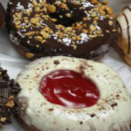
Another implemented method performs a randomly sized crop of the image:

And finally, we implemented a method to horizontally flip or mirror the image:

Note that all of these methods leverages the torchvision.transforms submodule. Now with these methods, we randomly sample an image in a category, randomly sample an augmentation method, and apply it to the sampled image to generate a new data instance to be added to the same category. We repeat this until the category reaches 500 data instances, then we perform this across all categories, reaching a total of 10000 training images. Finally, our data is cleaned up and ready to go.

Feature Selection & Image Compression with Principal Component Analysis (PCA)

Now that the dataset is ready to be used, we decided to do dimensionality reduction (in the form of image compression) using PCA in hope that the model would both run and train faster. This covers the unsupervised learning section of the project.

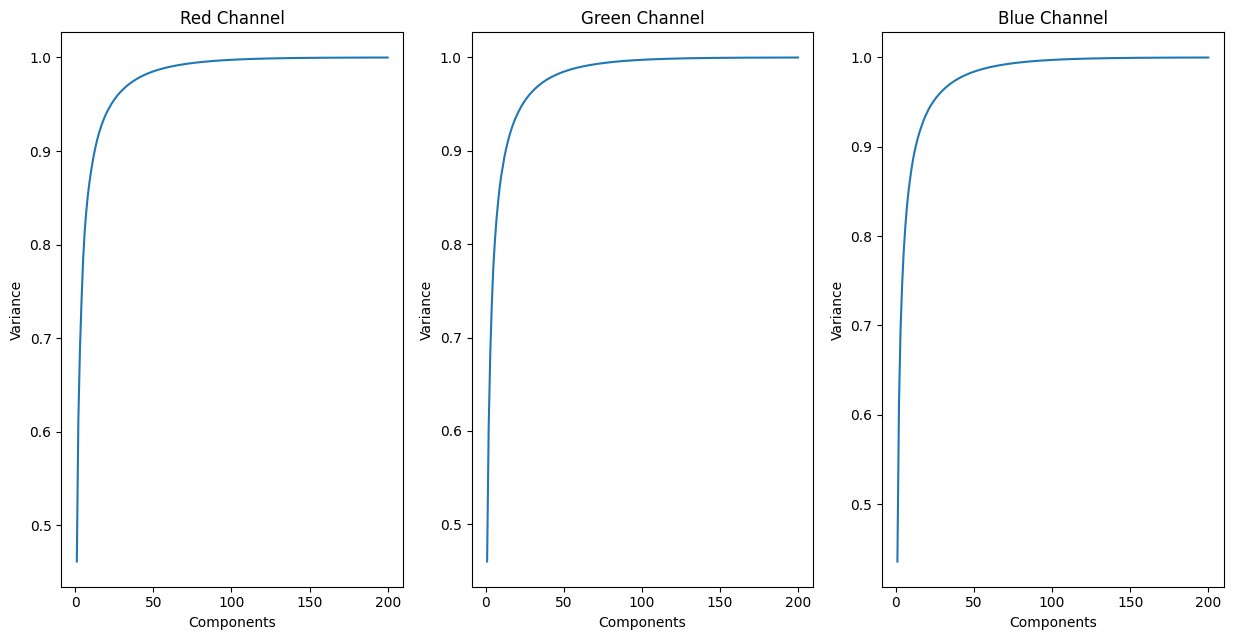
We wrote a method to apply PCA while choosing the number of components K. We verified this method by sampling some augmented images in our training set and applying the PCA method on different number of components (10, 25, 50, 100, 150, 200). Below are examples of our PCA method in action, along with the retained variance of each channel associated with each method call:

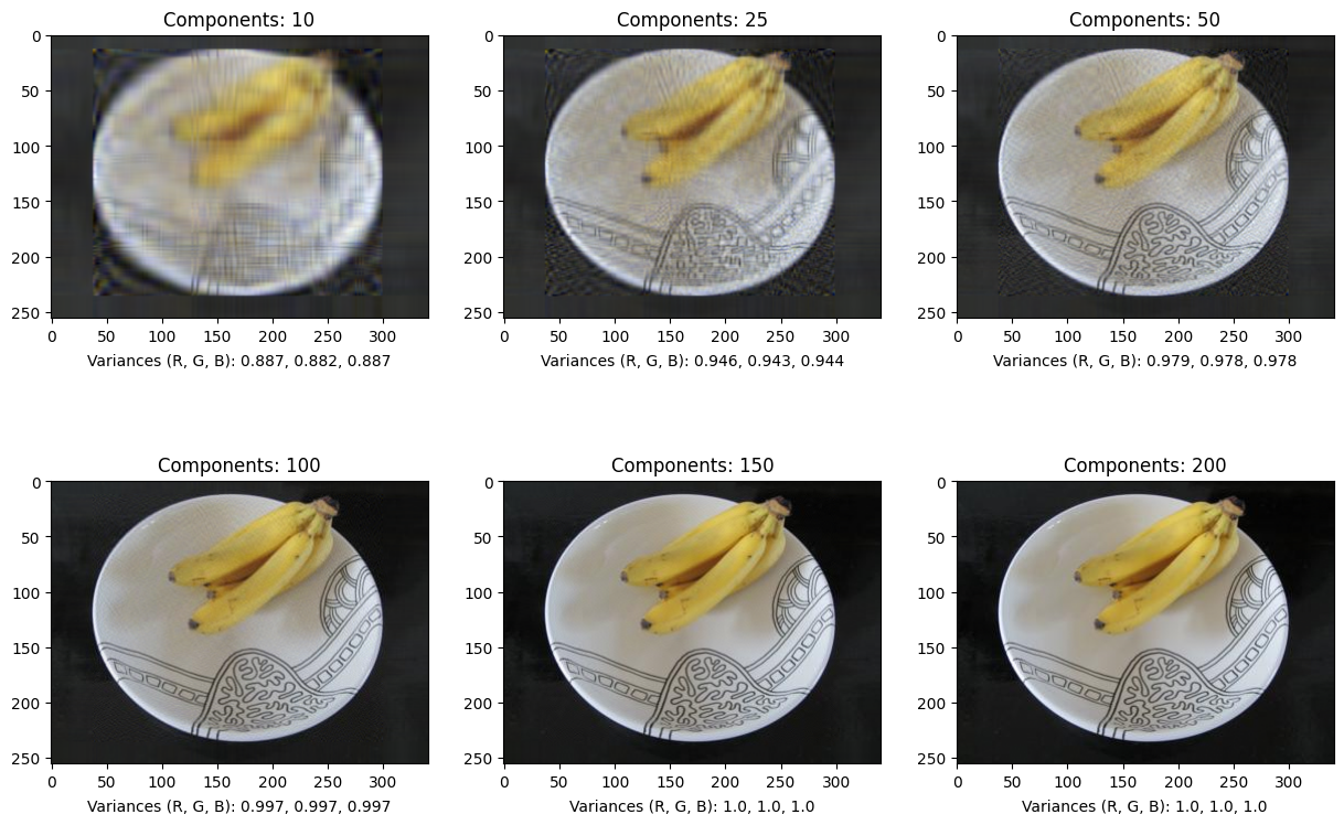
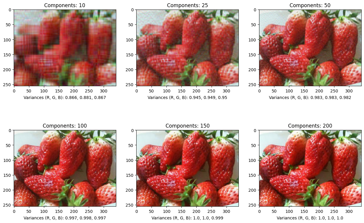
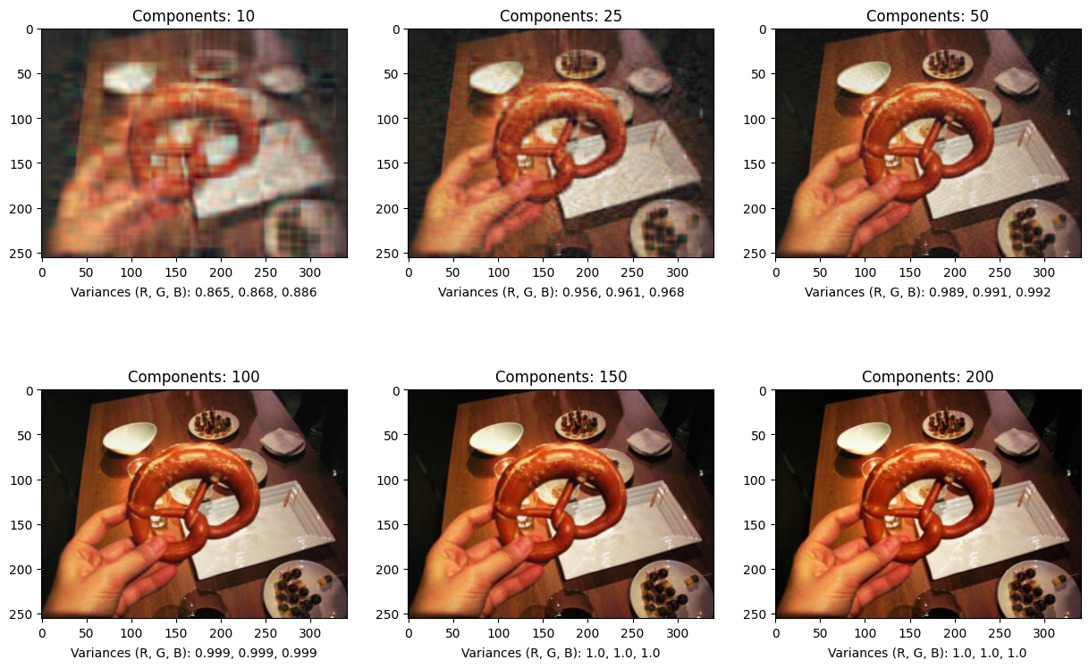
We can see that as the number of components increases, the images progressively become clearer, to the point where you are unable to tell the difference from the original image. At low levels of K, while the pictures have clearly lost detail, it is arguably not too difficult to make out the object in the image. To look at the trends of retained variance as we increased the number of retained components with PCA, we graphed our results for each color channel. We can see that the retained variance significantly drops after we have less than 40 components. Aiming to have at least 95% retained variance across all channels, choosing K to be around 50 looks to be optimal, although we wish to discover a better threshold for retained variance in our image compression technique.

Initial Attempts at Classification with Logistic Regression

Although we are eventually planning to use transfer learning, we decided to create a logistic regression model as a trial run after implementing PCA for image compression. For these trials, we decided to apply PCA on the training set with K = 100 (hoping to retain greater variance and detail in the image for our initial run). With the data augmentation, dimensionality reduction, and the logistic regression model in place, we got the following accuracies:

Logistic Regression, with PCA, with Augmentation	Accuracy
Training Accuracy	0.7596
Testing Accuracy	0.10189

Interestingly enough, the images without PCA applied have almost the same training and test accuracies.

Logistic Regression, w/o PCA, with Augmentation	Accuracy
Training Accuracy	0.7688
Testing Accuracy	0.10084

As expected, training and evaluating our logistic regression model on images with PCA applied took slightly faster compared to without (a few seconds of a difference, though this difference will likely be noticably larger for more complex classifier models we plan on using later on). Finally, for exploration, we decided to test the model against the original training dataset (without any data augmentation nor PCA):

Logistic Regression, w/o PCA, w/o Augmentation	Accuracy
Training Accuracy	0.7563
Testing Accuracy	0.10294

Note that all of these scores were derived via the LogisticRegression().scores() method, which returns the subset accuracy (requiring that the model classifies the correct label out of the possible 20).

While the training accuracies are decently high across the board, there is a big disparity with the test accuracy. This suggests that the model could be overfitting to the training data. However, even so, these training accuracies are not stellar and are inconsistent with their respective testing accuracies, suggesting that a logistic regression model is not adequate for non-trivial image classification unlike datasets such as MNIST [5]. As it stands, it is currently inconclusive whether our data augmentation and/or PCA have made classifying snacks in our dataset more or less effective. However, we hope that a CNN, such as ResNet or current state-of-the-art visual models, are able to tackle this classification task with less effort.

Midpoint Takeaways

While working on the midpoint, we have discovered interesting, possibly effective ideas that can be applied to our task that we unfortunately didn’t have the time to explore into before the deadline. One of these ideas is to utilize K-means or ISODATA as an unsupervised method to separate the training set into clusters. We can then manually observe these clusters and determine hidden unclean data instances inside the dataset, which we will promptly remove or specially augment. Also, in planning ahead with utilizing transfer learning for image classification, we discovered that such convolution/Max-Pooling layers from an existing trained model act as great feature selectors & extractors. In addition to this, we can use PCA on these extracted feature outputs, and attach afterward a classifier, such as another fully-connected neural network, random forest, or SVM. We hope to explore most, if not all, of these newfound ideas in our final project submission.

Contributions for Midpoint Proposal

Member	Contributions
Alex Tian	Github Page, Creating Graphs
Alwin Jin	PCA, Logistic Regression
Daniel You	Principal Component Analysis
Richard So	Dataset Loading, PCA, Github Page
Varshini Chinta	Data Augmentation

References

[1] Roopnarine, P. D. (2014). Humans are apex predators. Proceedings of the National Academy of Sciences, 111(9), E796-E796.

[2] https://huggingface.co/datasets/Matthijs/snacks

[3] He, K., Zhang, X., Ren, S., & Sun, J. (2016). Deep residual learning for image recognition. In Proceedings of the IEEE conference on computer vision and pattern recognition (pp. 770-778).

[4] A. Kuznetsova, H. Rom, N. Alldrin, J. Uijlings, I. Krasin, J. Pont-Tuset, S. Kamali, S. Popov, M. Malloci, A. Kolesnikov, T. Duerig, and V. Ferrari. The Open Images Dataset V4: Unified image classification, object detection, and visual relationship detection at scale. IJCV, 2020.

[5] https://github.com/nst/MNIST