Final Report Submission
Table of Contents
Introduction
Food stands for any item that serves as a source of nutrition for a living organism. Being omnivores and apex predators, humans eat foods that come in all sorts of shapes, sizes, textures, and flavors [1]. Similarly, humans have vastly different preferences for which foods they’d rather consume. Still, there exists foods that are ubiquitously popular across the world. Ask any person if they are willing to pass up a sweet scoop of ice cream or perhaps a juicy, well-seasoned hot dog.
Generally, humans are quick to identify and fixate upon their favorite foods in
their visual field. The Mattijs/snacks dataset is a collection of images of
popular food items derived from the Google Open Images dataset, and is
accompanied in textbooks such as Machine Learning by Tutorials [2, 4].
Give a human this dataset, and they can effortlessly classify which food is which. However,
many people who are visually impaired may struggle with the crucial task of
identifying what they are consuming. A program to identify everyday foods, such
as apples or cookies, may prove to be useful for such individuals.
Problem Definition
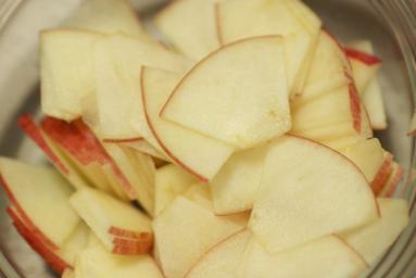
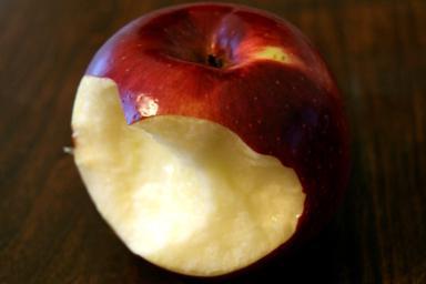
Identifying food items purely from visual appearance is surprisingly
non-trivial. Here are examples of “apples” in the snacks dataset:
 |
 |
 |
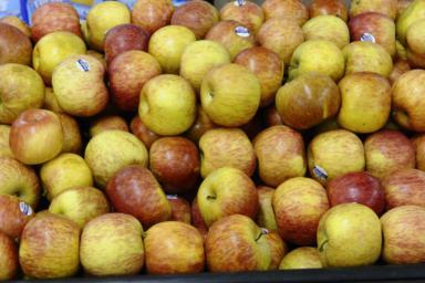 |
Even with just one label, “apples” come in different forms, colors, and counts.
Our objective is to make a machine learning model that can accurately classify
the main type of food/snack apparent in an input image while generalizing to the
variety of appearances that such an item can take. Since the project proposal,
we have decided to move forward with the classification problem regarding the
snacks dataset.
Data Collection
The Mattijs/snacks dataset is available in the Hugging Face Datasets Hub
[2]. Therefore, there was no manual data collection required on our
part. We leveraged the Hugging Face Datasets library to download the dataset
from the Hub. The returned object is a wrapper of an underlying Apache Arrow
dataset containing all images and corresponding labels that we utilize heavily
throughout the project.
Methods
Dataset Preparation & Augmentation
The snacks dataset has 20 different class labels of various different foods.
The classes are as follows: ‘apple’, ‘banana’, ‘cake’, ‘candy’, ‘carrot’,
‘cookie’, ‘doughnut’, ‘grape’, ‘hot dog’, ‘ice cream’, ‘juice’, ‘muffin’,
‘orange’, ‘pineapple’, ‘popcorn’, ‘pretzel’, ‘salad’, ‘strawberry’, ‘waffle’,
‘watermelon’.
The photos in the dataset are of various dimensions. However, the images were scaled by the authors of the dataset such that the smallest dimension is 256 pixels. The dataset has already been divided into a train, validation, and test split. Below is the number of data instances for each split that came with the dataset:
| Set/Split | Count |
| Train | 4838 |
| Validation | 955 |
| Test | 952 |
| Total | 6745 |
Here is the breakdown of the counts of examples per label:
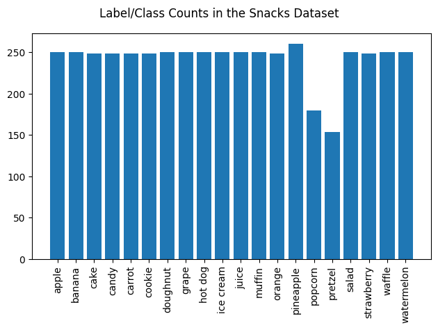
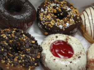
Most of the classes have 250 examples, with the exception of ‘popcorn’ and ‘pretzel’. Ideally, we’d want the number of images in each class to be even. Additionally, to help generalize the model to snacks of different forms and sizes that appear at varying areas of the image frame (as discussed above), we decided to augment our training split with slight modifications, or transformations. Some of these transformations involve scaling, rotating, cropping, and mirroring. For instance, take the following image, originally sampled from the training set:

We implement a scaling method, which simply makes the image smaller or larger on a uniform scale between 0.8 times and 1.2 times.
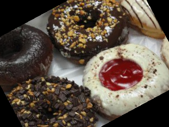
Our rotation method rotates the image up to 30 degrees counter/clockwise.
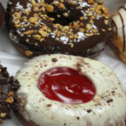
Another implemented method performs a randomly sized crop of the image that preserves up to 50% of the original image size:
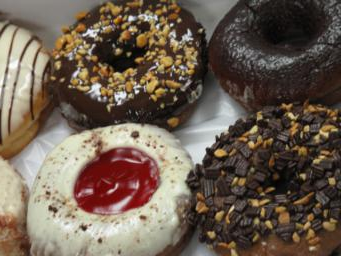
And finally, we implemented a method to horizontally flip (mirror) the image:
All of these methods leverages the torchvision.transforms submodule. Now with
these methods, we randomly sample an image in a category, randomly sample an
augmentation method from this pool, and apply it to the sampled image to
generate a new data instance to be added to the same category. We repeat this
until the category reaches 300 data instances, then we perform this across all
categories, reaching a total of 6000 training images.
Feature Reduction & Image Compression with Principal Component Analysis (PCA)
Principal Component Analysis (PCA) is a powerful dimensionality reduction
method that has expansive applications in the space of Machine
Learning[6]. It assists in reducing the feature space of a dataset in
order to assist supervised learning models with converging more efficiently to
minimal loss (and maximal accuracy). A known, elementary approach to image
classification (seen in Assignment 3) is to flatten the image, apply
PCA on the flattened vector, and pass this to a classifier like
sklearn.linear_model.LogisticRegression to train on.
However, PCA is also known for being an effective method for image compression because of it’s innate ability to preserve as much information of the original data with the number of components the algorithm is allowed to worked with. Arguably, PCA image compression helps reduce the details of an image to ones that are most essential to identifying elements of the image itself. Thus, for this project, we will incorporate both of these applications of PCA into our methodology, covering our unsupervised learning method of choice.
We wrote a method to apply PCA while choosing the number of components K. We
verified this method by sampling some augmented images in our training set and
applying the PCA method on different number of components (10, 25, 50, 100,
150, 200). We utilize the sklearn.decomposition.PCA (and IncrementalPCA in
situations where memory is scarce) implementations in order to perform PCA
image compression. For each image, we split and run PCA runs over the three
color channels, and finally reconstruct the image to yield the compressed
image, and repeat for all images in the dataset. Below are examples of our PCA
method in action, along with the retained variance of each channel associated
with each method call:
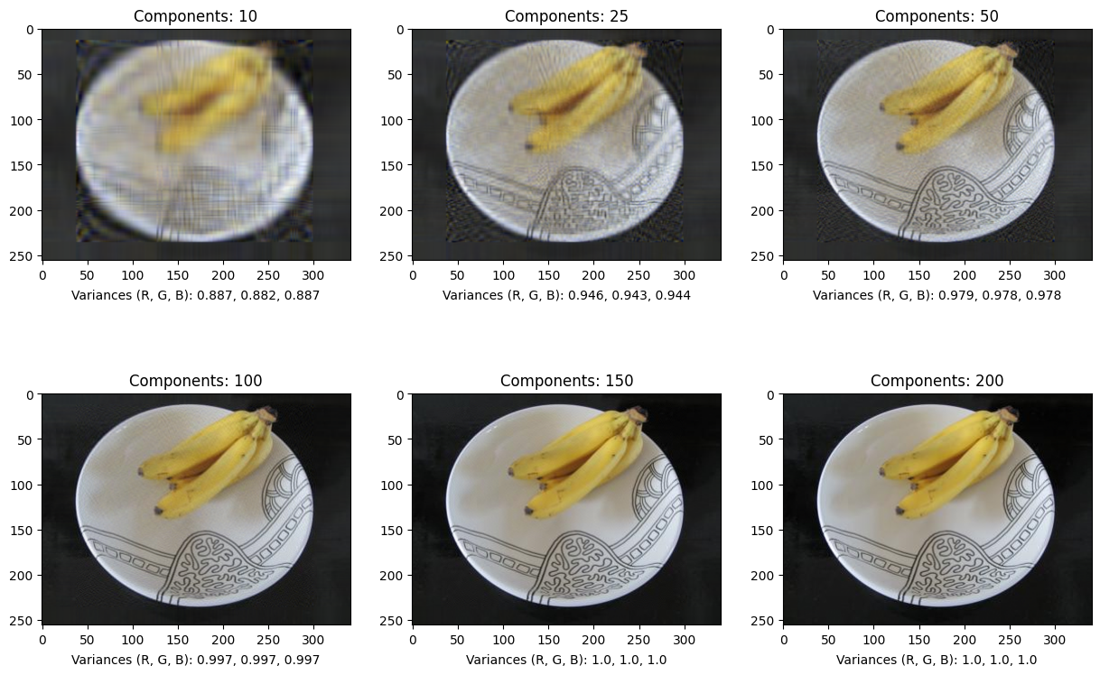
K = 200 seems to be identical to the original image, while K = 10 holds
significantly less resemblance. Clearly, there is a selection for K that
balances the preservation of features from the original image while reducing
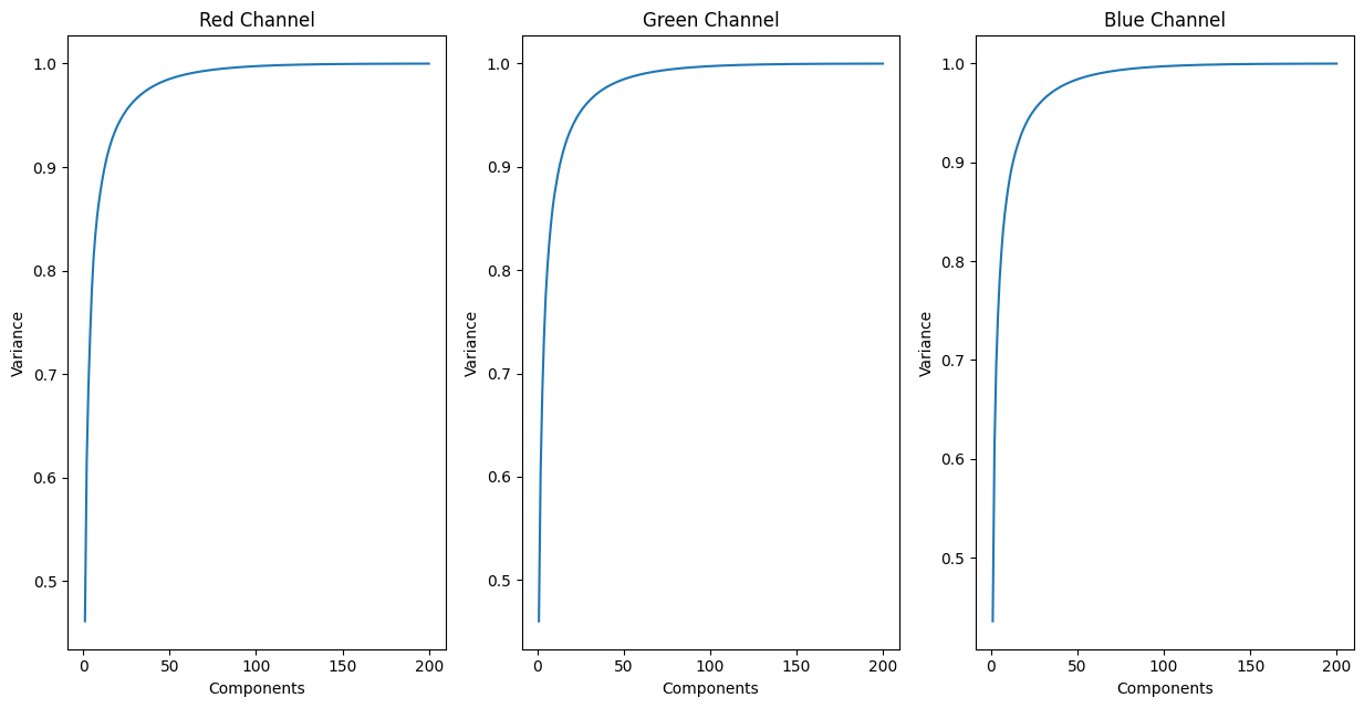
its unnecessary details and speeding training and/or evaluation times. We do
this by observing the retained variance as we increase K for our PCA
implementation, for each channel color. Through this, we find that the retained
variance significantly drops after we have less than 40 components. Aiming to
have at least 95% retained variance across all channels, choosing K to be
around 75-100 looks to be the most optimal.
Classification Models
Until now, this report has been concerned with the preprocessing and augmentation of the dataset. Our ultimate goal is to accurately classify snacks that exist in an image. We propose multiple supervised learning methods that will bring us closer to this goal:
-
LR: Standard Logistic Regression on flattened images -
LR-PCAr: Logistic Regression on flattened images reduced by PCA (K = 500) -
LR-PCAc: Logistic Regression on images flattened after PCA image compression (K = 100) -
ResNet: Residual Network, transfer learned from the ImageNet-1k dataset, trained on regular images -
ResNet-PCAc: Residual Network, transfer learned from ImageNet-1k, trained on PCA-compressed images (K = 75) -
ViT: Vision Transformer, transfer learned from the ImageNet-1k (regular images) -
RegNet: RegNet, transfer learned from the ImageNet-1k (regular images)
Note that, although subtle, there is a difference between LR-PCAc and
LR-PCAr. The latter applies PCA in a more “regular” fashion, reducing the
amount of features from [height * width * 3] to K (500). The former
flattens and trains on images that have already been compressed with our PCA
image compression technique outlined above using 100 components for each
channel. Additionally, due to memory limitations, images had to be scaled to
128-by-128 squares before flattening for LR-PCAr training. Both methods of
logistic regression will be based on the
sklearn.linear_model.LogisticRegression implementation.
Half of our models are Convolutional Neural Networks (CNNs), in which a
significant (initial) portion of its layers have sliding kernels to help
extract edge, corner, and pattern features from image data [10]. These
kernels also preserve spatial information across colors, unlike the LR models
where all pixels must be flattened into a one-dimensional vector per example.
Transfer learning is a technique where a model trained on a certain task is ported, retrained (usually altering just the later layers of the network), and evaluated in a slightly different (sub)task [9]. This is a common technique among machine/deep learning practitioners, especially in the domain of image classification, and is quite effective in cases where the training dataset for the task is relatively small. Considering that our augment dataset is around 6000 images, and some popular image datasets like ImageNet-1k contains over 1 million images, we found transfer learning to be a very appropriate technique to apply for our task.
ResNet[3] is an extremely popular Convolutional Neural Network
renowned for its approach to the vanishing gradient problem, which is prevalent
for very deep and complex neural networks. Essentially, backpropogation issues
smaller weight changes as the network is updated back to the initial layers
to the point where the first layers of the model struggles profusely to
converge. The result is to introduce shortcut connections where the
identity of a layer is added to an output two layers deeper so that the
gradients from the update phase do not diminish as quickly. We used
ResNet (torchvision.models.resnet101) on the original set of augmented
images along with another set of augmented and PCA-compressed images
(ResNet-PCAc).
ViT, or Vision Transformer [7], is a novel method that borrows the
well-known Transformer architecture seen in applications of natural language
processing and brings it into the realm of computer vision and image
classification. Transformers are known to be very computationally efficient,
retaining magnitudes more model parameters with the same computational
(training) time and cost. ViT has been found to be successful once trained on
a massive amounts of data, surpassing ResNet in many image tasks with a
seemingly unconventional architecture. This is a driving reason why we decided
to transfer learn ViT for our classification task. Specifically, we chose the
torchvision.models.vit_l_16 model (Large ViT with a 16-by-16 input patch
size).
RegNet [8] is the result of an iterative process of shrinking an
initial exhaustive, parametrized set of network architectures and seeking a
subset (or “family”) of optimal network architectures. The architecture is made
up of residual blocks (like ResNet), however, its depth and width can be
dynamically adjusted with a quantized linear function, meaning that RegNet
can be adjusted for faster performance or better accuracy. RegNet has shown
to beat MobileNet, EfficientNet, and ResNet, all in their own domains (in
terms of accuracy), just by adjusting RegNet accordingly. We evaluate how
well torchvision.models.regnet_y_32gf, one of the larger models among the
family, performs as a feature extractor for snacks.
For all models (feature extractors) that we utilized for this project, we performed a variant of transfer learning as detailed below: we froze the weights of the convolutional layers, otherwise known as the feature extractors, since they have been trained extensively on the ImageNet-1k dataset. We attached a small fully-connected sequential module to the end of each CNN to act as our actual classifier that we train on, identical across all CNNs (and Vision Transformer), defined as following:
nn.Sequential(
    nn.Linear(output_features, 512),
    nn.LeakyReLU(),
    nn.Dropout(.2),
    nn.Linear(512, 20)
)
where output_features is the number of features from the feature extractor,
varying across the architectures. After trial and error, we used a learning
rate of 1e-4 with the torch.optim.Adam optimizer each network. We do not
have a set epoch count when training these models, instead opting for an
EarlyStopping callback with a patience of 3 on the validation loss (meaning
that the model stops training once the validation loss does not decrease for
more than three epochs). The training and evaluation of these models were
implemented with PyTorch with a high-level API wrapper PyTorch Lightning.
Results
Logistic Regression
We use the model.score() Scikit-Learn method to determine the accuracy of our
two Logistic Regression models. Under the hood, this method computes the mean
accuracy (percentage examples predicted correctly) of the model given a pair of
training examples and labels. The following are our accuracy values for our LR
models:
| Model Type | Training Accuracy | Testing Accuracy |
LR |
0.7688 | 0.10084 |
LR-PCAr |
0.4948 | 0.07142 |
LR-PCAc |
0.7596 | 0.10189 |
Clearly, the scores for the logistic regression models are extremely low. This
is because of the large amount of features images have. For images, since we
are using logistic regression, we must flatten each of the images before
inputting into the model. Thus, using 256-by-256 images, there are a total of
256 * 256 * 3 = 200,000 features. Using this many features is nearly
guaranteed to overfit, and thus we see acceptable training scores but
completely unacceptable testing scores. We also experience a dip in performance
for LR-PCAr compared to the other two LR models because we had to shrink
the images down to 128-by-128 squares, giving this model a quarter of the amount
of features to work with compared to the other models even before PCA
dimensionality reduction.
Note that the LR-PCAc model performs slightly better as expected, since PCA
reduces the number of features for each image. However, the model still
performs very poorly on the test set. This low accuracy can also be attributed
to overfitting, as it is possible that setting k = 500 still yields too many
features. In addition, the model might be learning from incorrect things. For
example, many of the training images contain noise, such as humans holding
snacks or other background features. The models are learning to recognize these
background features and not the actual snack in the image frame, resulting in
poor overall performance on the test set that has less background features.
Due to the appalling performance of the LR models, we found it insignificant
to dive deeper into greater detail of their metrics. A theoretical analysis on
why PCAr did not help significantly for this task will be covered in the
discussion section.
Transfer Learned Models
For our transfer learned models, we used the recall_score,
precision_score, and f1_score methods provided within sklearn.metrics.
Below are top 1 performances on the testing dataset:
| Model Type | Recall | Precision | F1-score |
ResNet |
.87710 | .88165 | .87753 |
ResNet-PCAc |
.86554 | .87180 | .86637 |
ViT |
.92857 | .93140 | .92844 |
RegNet |
.90651 | .90850 | .90625 |
As expected, the neural network approach vastly outperforms logistic
regression. Taking a look at the two convolutional neural network models,
ResNet and ResNet-PCAc, we observe good accuracies on both. CNNs are able
to perform feature extraction on their own due to their sliding kernels. The
convolutions serve to essentially blur images, resulting in less overall
features and reducing the risk of overfitting. In turn, this allows the model
to learn generic features in the image, instead of pixel by pixel like logistic
regression does. Additionally, we see that the PCA variant of ResNet actually
performs worse than the non-PCA variant. This is because of the compression
effect CNNs have, meaning that in this case, more features is better than
limiting features with PCA.
Vision Transformer, ViT, performs the best out of all the models, even
surpassing RegNet. The high accuracy can be attributed to the self-attention
mechanism of transformers. Attention allows the model to focus on important
parts of images, which is good for combatting the background noise in images.
For example, when working to detect a picture of an apple on a picnic bench,
the attention mechanism will give more weight to the apple and less weight to
the picnic bench. Thus, we see the Vision Transformer outperforming the CNNs,
as CNNs do not have attention mechanisms and likely are also learning from
image backgrounds instead of just the subject. Considering that CNNs have been
the de-facto standard for computer vision models for decades, this finding is
an upset, like a happy underdog story for Vision Transformer. However, it
should be acknowledged that both ViT and RegNet were introduced a
half-decade after ResNet. It is impressive that ResNet is holding very well
on its own, thus showing the power of the residual blocks that its authors had
coined.
We also evaluated the top 3 and top 5 accuracies of each model, meaning that the model would have considered to classify an example correctly if any of its largest 3 or 5 predictions match the ground truth, respectively:
| Model Type | Top 3 | Top 5 |
ResNet |
.97584 | .99055 |
ResNet-PCAc |
.97059 | .98634 |
ViT |
.98214 | .99055 |
RegNet |
.97584 | .98950 |
Once we loosen the guidelines for what is “correct”, as expected, the
accuracies skyrocket. Amazingly, all models were at least 97% accurate in
their top three predictions out of 20 categories. As a side note, it is
interesting that ResNet surpasses RegNet to match ViT regarding top 5
accuracy.
Class/Label-level Visualizations
For all models, we constructed a confusion matrix on the testing dataset to determine which classes were the weak points for each model:
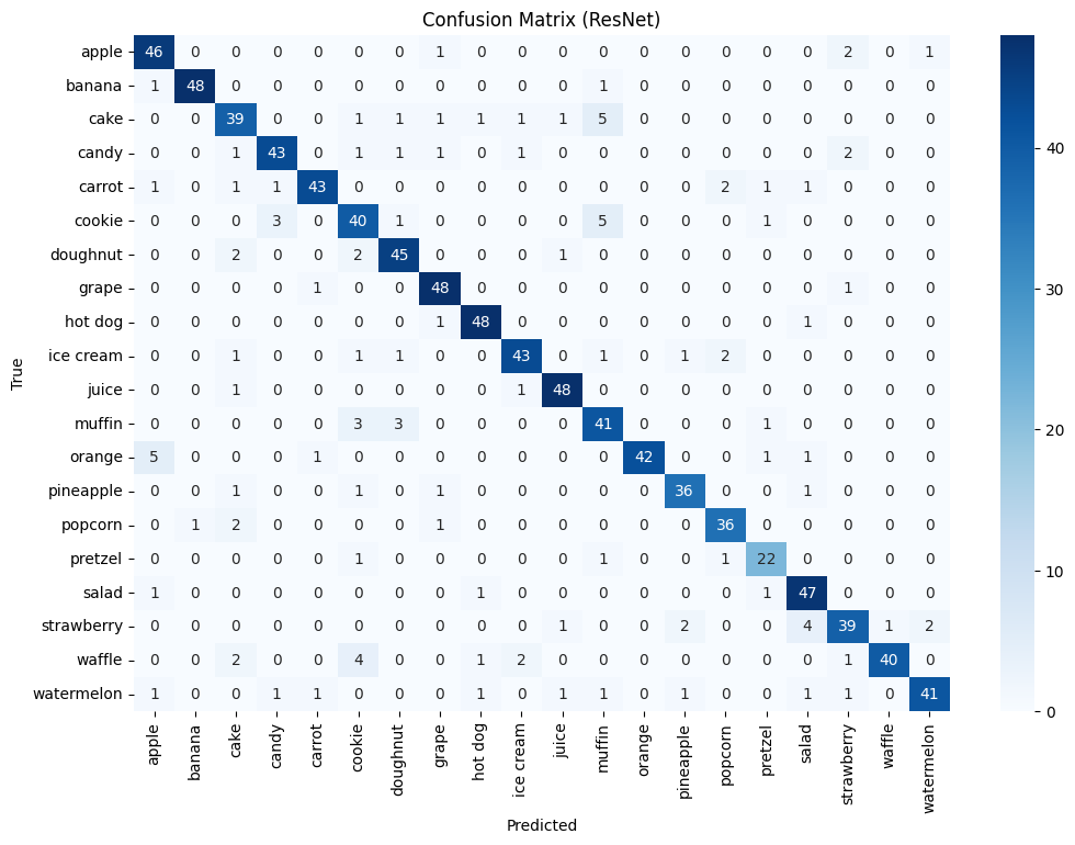

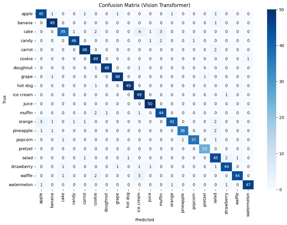
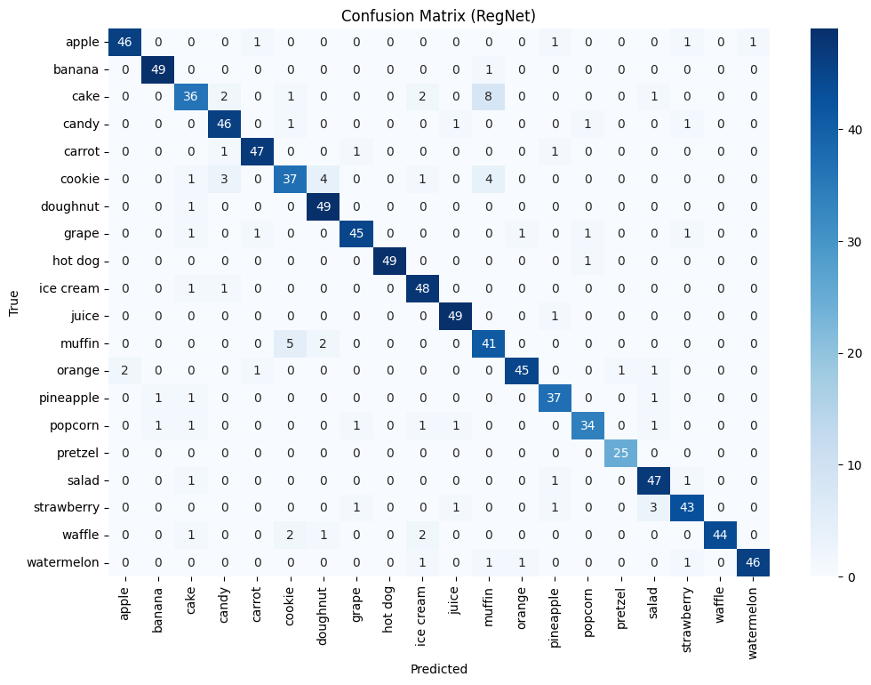
There are some shared instances where the model incorrectly predicted an orange to be an apple. Since we did not apply a hue augment to the dataset, these could be due to some dirty data in the testing set, where there might be incorrect/swapped labels. Other possibilities include the fact that there could be instances of both apples and oranges in the image frame, or that the orange in the example has an uncommon color that is not seen often in the training or validation set, causing the models to believe that it is an apple. All models have a slight mix up cakes with muffins and cookies, which in retrospect seems reasonable because all of these snacks are baked goods. Otherwise, the performances of all models were very solid and satisfactory.
We also measured the precision, recall, and F1-score of each predicted class, for each model:
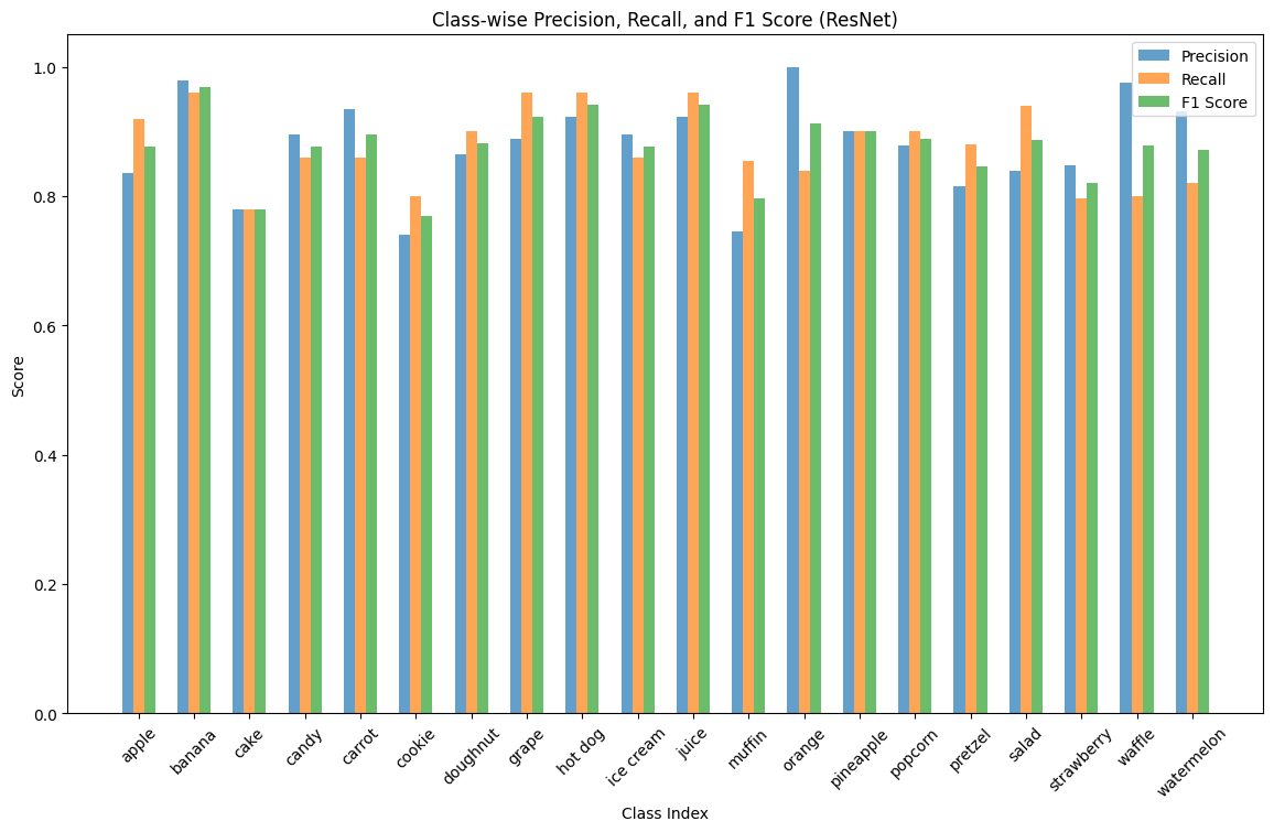
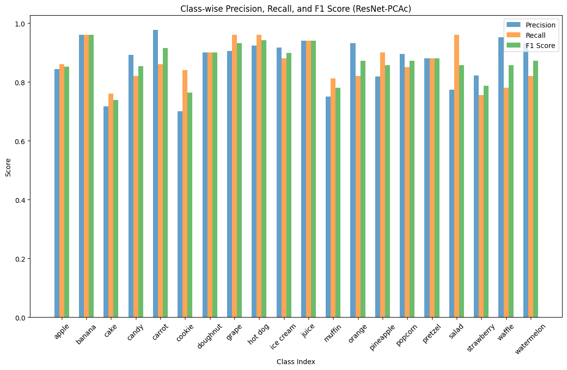
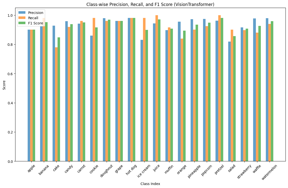
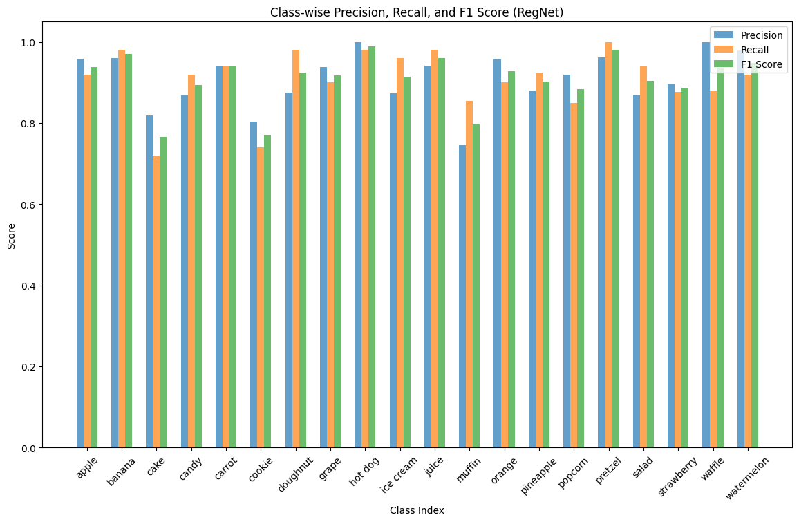
Again, we observe the unanimous small dip in performance in muffins, cakes, and cookies, though we also see that some models uncommonly struggle with classifying salads or strawberries. Ultimately, we are happy with the results of our application of transfer learning onto the task.
Discussion
Why does Logistic Regression and PCA fail?
In Assignment 3 of this course, we explored how applying PCA on flattened
images can help speed up training for a LogisticRegression model with simple
mask detection. We attempt to mirror this approach with our LR-PCAr model,
yet we found sub-par results. Aside from the necessity of scaling the images
down to a quarter of their original size to fit in memory (even with the use
of IncrementalPCA), we attempted at visualizing the dataset with PCA
reduction using two components to see if there exists any evidence of class
boundaries:
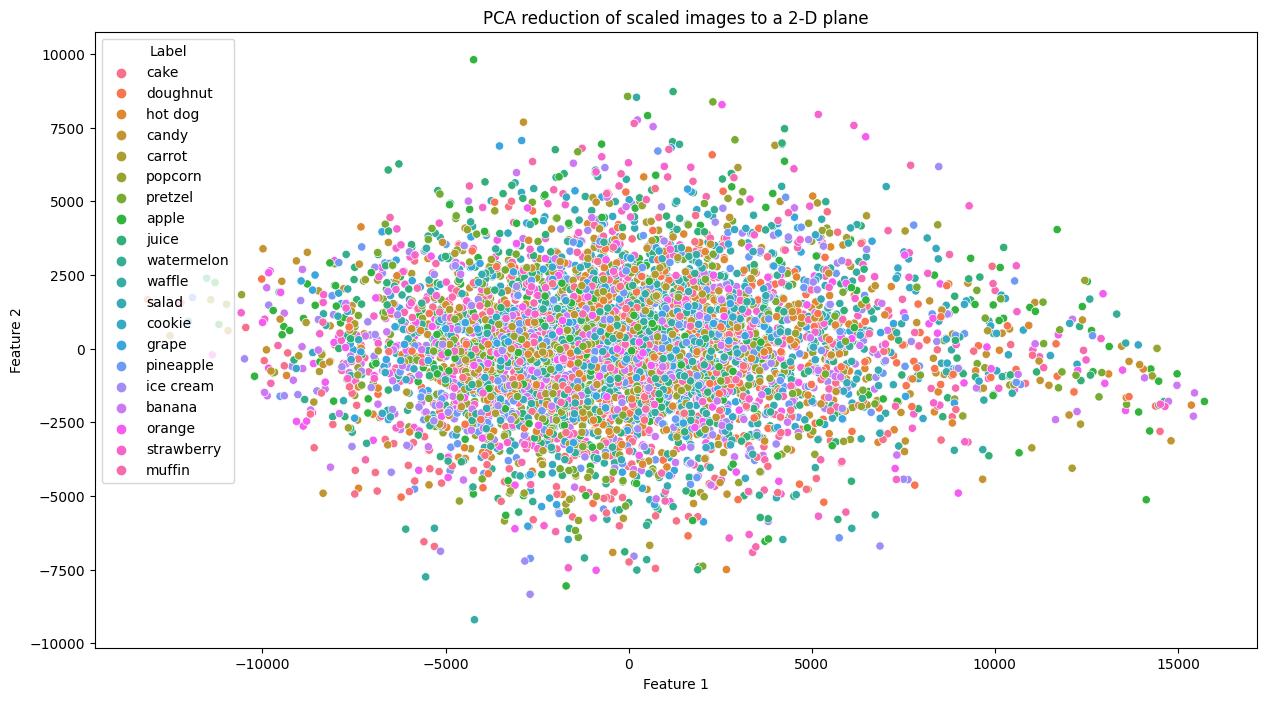
Our reduction of the dataset into two components/features has made it virtually
impossible to deduce any of the 20 classes, a stark contrast to our Assignment
3 exploration. Even if we consider that two components is a grand exaggeration
of the issue at hand, the results from the previous section show that this
problem still exists at higher K, or even when PCA is not in use. As a
result, Logistic Regression is not adequate in capturing the complexity of this
classification problem.
Wrapping Up
In conclusion, we have observed numerous models in our pursuit to classify
snacks in images as accurately as possible. We see that Logistic Regression
models are not ideal for this task, especially if there are many different
classes to learn and classify. In multiple portions of our project, we employed
several use cases of Principal Component Analysis in an attempt to reduce the
complexity of the data we were working with. However, we eventually found CNN
and Transformer-based feature extractors to be more ideal for this feature
extraction and reduction task. We found ViT to be the best feature extraction
model out of all the others we have tested, thus validating its
state-of-the-art status in academia. Overall, we found this project to be very
fun and eye-opening of current, effective techniques in the domain of image
classification tasks.
Contributions for Final Proposal
Although all members of the group contributed to fill positions for each other whenever necessary, the following is a mapping to the most important contribution made by each team member:
| Member | Contributions |
| Richard So | Model Implementation, Results Metrics, Final Report |
| Daniel You | Video Presentation |
| Alex Tian | Video Presentation |
| Alwin Jin | Model Implementation, Final Report |
| Varshini Chinta | Results Metrics, Visualization |
Timeline Chart
Or view the spreadsheet here
References
[1] Roopnarine, P. D. (2014). Humans are apex predators. Proceedings of the National Academy of Sciences, 111(9), E796-E796.
[2] https://huggingface.co/datasets/Matthijs/snacks
[3] He, K., Zhang, X., Ren, S., & Sun, J. (2016). Deep residual learning for image recognition. In Proceedings of the IEEE conference on computer vision and pattern recognition (pp. 770-778).
[4] A. Kuznetsova, H. Rom, N. Alldrin, J. Uijlings, I. Krasin, J. Pont-Tuset, S. Kamali, S. Popov, M. Malloci, A. Kolesnikov, T. Duerig, and V. Ferrari. The Open Images Dataset V4: Unified image classification, object detection, and visual relationship detection at scale. IJCV, 2020.
[5] https://github.com/nst/MNIST
[6] https://mahdi-roozbahani.github.io/CS46417641-fall2023/course/14-dimension-reduction.pdf
[7] Dosovitskiy, A., Beyer, L., Kolesnikov, A., Weissenborn, D., Zhai, X., Unterthiner, T., … & Houlsby, N. (2020). An image is worth 16x16 words: Transformers for image recognition at scale. arXiv preprint arXiv:2010.11929.
[8] Radosavovic, I., Kosaraju, R. P., Girshick, R., He, K., & Dollár, P. (2020). Designing network design spaces. In Proceedings of the IEEE/CVF conference on computer vision and pattern recognition (pp. 10428-10436).
[9] https://machinelearningmastery.com/transfer-learning-for-deep-learning/
[10] https://mahdi-roozbahani.github.io/CS46417641-fall2023/course/19-neural-network-cnn.pdf